Stock market data have been heavily investigated to explore the trend of securities’ return and their risk. Factor models are the most canonical and widely used models for asset pricing and security selection for portfolios. In this project, we aim to utilize various factors and a linear model to predict the medium-term return and risk of a particular stock. The datasets include the historical prices of the stocks in the US stock market and their corresponding fundamentals in the same period.
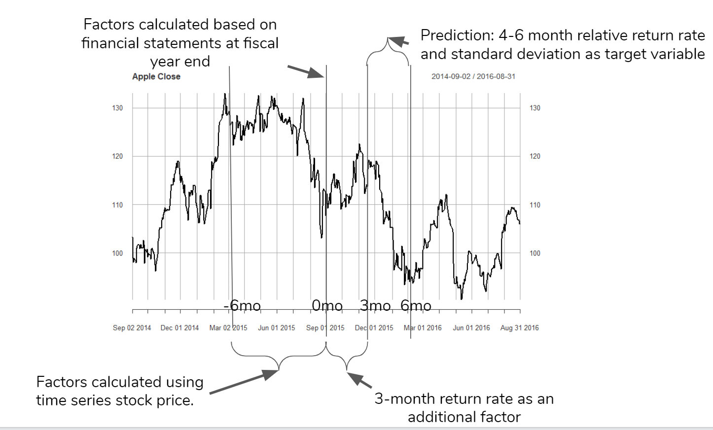
The logic can be visualized in the plot above: for each firm at the end of its fiscal year, we regard it as one observation point. Taking Apple as an example, its fiscal year ends every September. We build factors based on fundamentals of the past fiscal year and the past half-year stock price. Since the financial statement is released 2-3 months after the fiscal year ends, we can also have the three months return rate as an additional variable. Finally we predict the return rate and risk of next quarter(4-6 months after the fiscal year ends).
Factors
Some of the factors we are theoretically based on this Barra US Equity Model presented MSCI, which can be found at http://cslt.riit.tsinghua.edu.cn/mediawiki/images/4/47/MSCI-USE4-201109.pdf. The construction of the factors are described below:
1. Industrial Factor
Use the ‘GICS’ factor in securities.csv. Use each industry as a dummy factor.
2. Risk Factor
(1) Size
Natural log of market capitalization
Formula:
cap: we use the estimated share outstanding(in fundementals.csv) * stock price(on the last day fof the fiscal year, merged from prices.csv)
(2) BETA
Beta is a concept that measures the expected move in a stock relative to movements in the overall market. A beta greater than 1.0 suggests that the stock is more volatile than the broader market, and a beta less than 1.0 indicates a stock with lower volatility.
Formula:
: one-year treasury rate
: S&P 500 return - r_t
: Stock price return
(3) Momentum
Measures the velocity of price changes in a stock.
Formula:
is an exponential weight with a half-life of 63 trading days.
(4) Residual Volatility
Defition: 0.74 · DASTD + 0.16 · CMRA + 0.10 · HSIGMA
DASTD: Daily Standard Deviation
CMRA: Cumulative Range
HSIGMA:
(5) Nonlinear Size
Cube of natural log of market capitalization
Formula:
cub =
Size =
(6) Book-to-price
Formula:
(7) Earning Yields
EY = (0.21CETOP + 0.11ETOP)/0.32
where:
CETOP = Earnings Per Share/Share Price
ETOP = Net Income/Size
(8) Leverage
LEV = 0.38 · MLEV + 0.35 · DTOA + 0.27 · BLEV
where:
Market leverage:
MLEV = (Size + Longterm Debt)/Size}
Debt-to-asset:
DTOA = (Total Liabilities)/Total Asset
Book leverage:
BLEV = (Total Equity+Longterm Debt)/Total Equity
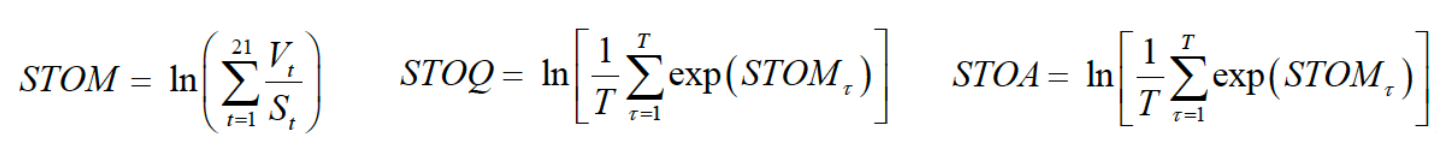
Liquidity:
3. Other Factors that Can Directly Add
Current Ratio
Quick Ratio
Profit Margin
After Tax ROE
Models
After the financial reports are released, we want to give investors a general sense of how the stocks are going to perform in the next quarter. So, we have chosen two target variables, one measures the profitability, the other measures the risk. For profitability, we chose quarterly return relative to market after three months of releasing financial reports. For risk, we chose the standard deviation of daily returns. This metric measures how volatile the stocks are, and it’s a common approach in finance to quantify the risk.
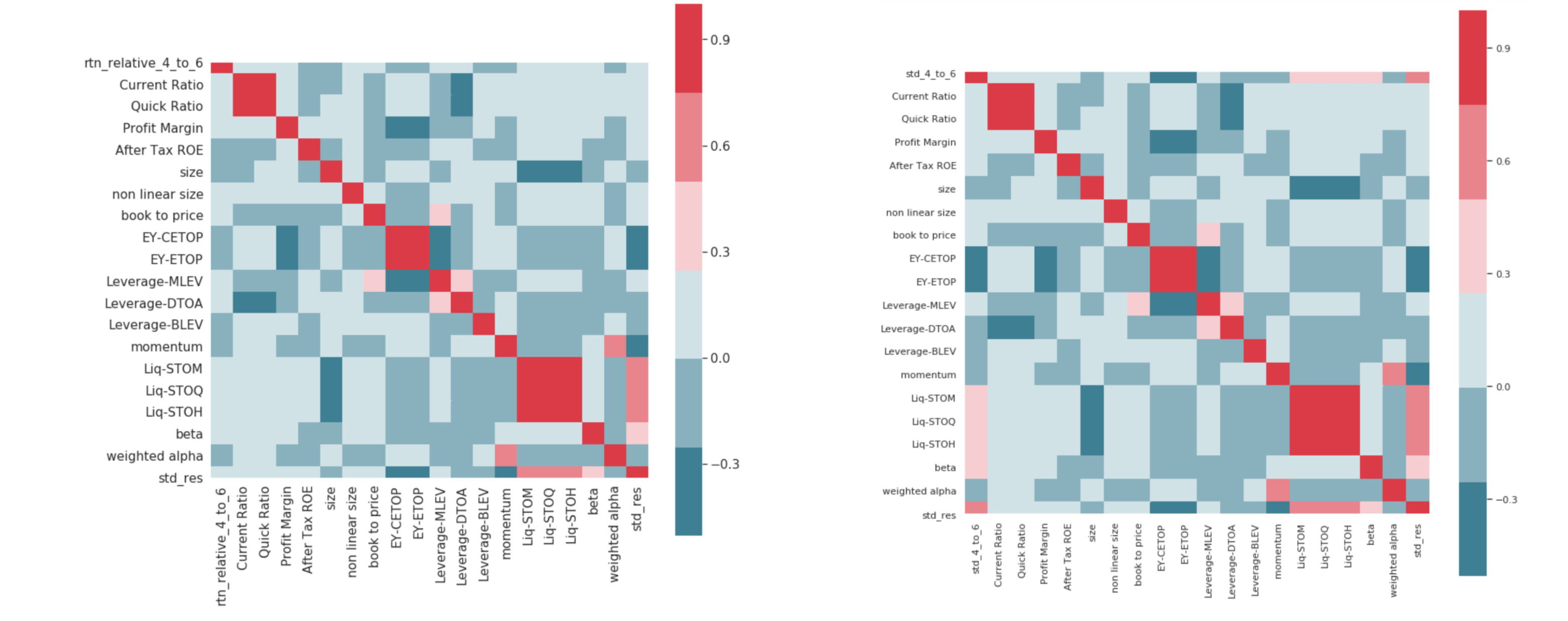
The two heatmap focuses on the relationship between two target variables and the factors. These two correlation matrices are the same but different in their first row/column. The first row of the left one here is the quarterly return. The right one here is the daily return standard deviation. We can find that daily return standard deviation is more correlated with the factors, as we can see more dark blue and red in the first row. So we expect a more accurate prediction for std measuring the risk.
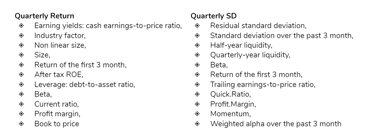
We first used step AIC to perform feature selection. The AIC criterion is defined for a large class of models fit by maximum likelihood. The penalty increases as the number of predictors in the model increases, and this is intended to adjust for the corresponding decrease in training RSS. As a consequence, the AIC statistic tends to take on a small value for models with a low test error, so when determining which of a set of models is best, we choose the model with the lowest AIC value.The plot belows shows the features selected based on step AIC algorithm,for quarterly return and quarterly variance, respectively. Such features will be further used as the independent variables for different models.
In addition to simple linear regression, three models, elastic-net regression, ridge regression and k-nearest neighbors were trained in seeking for a better prediction performance and interpretable results. RMSE was used as the metrics to measure the average squared error. Furthermore, a five-fold cross validation was implemented during the training: each fold will be sequentially used as a test set to measure the performance of the model trained by the training set to prevent overfitting on the training data.
Results
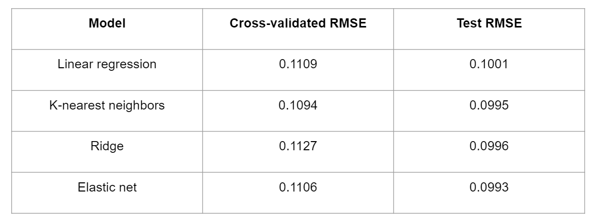
The results for quarterly return are presented in the table above. Elastic-net regression, ridge regression and k-nearest neighbors perform slightly better than linear regression as they have smaller test RMSEs. All models have test RMSEs around 10%, and elastic net has a small advantage over KNN and ridge regression with an RMSE of 9.93%.
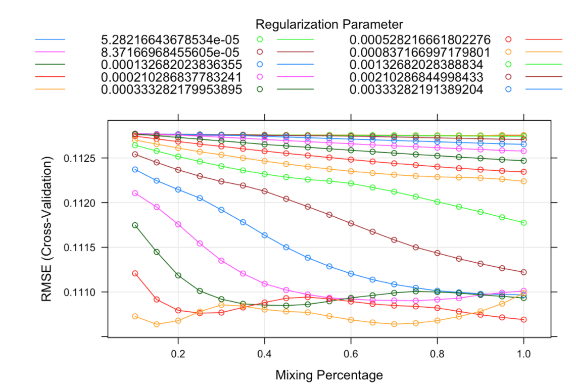
The elastic-net model is further investigated for parameter interpretation. As shown in the plot above, the horizontal axis represents the mixing percentage as known as the parameter alpha in the elastic-net regression. The vertical axis represents cross-validated RMSE, and each line represents a different lambda. The orange line at the bottom with a mixing percentage of 0.15 has the smallest RMSE. This indicates that our best model is an elastic net regularization with alpha 0.15 and lambda 0.021.
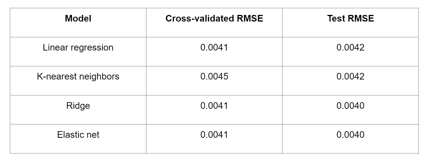
The table above shows the results for quarterly standard deviation with the same four models used. First it is clear that KNN performed the worst among all the models. Linear regression got the same result as ridge and elastic-net in cross-validation, with a slight decrease in RMSE in the testing data.
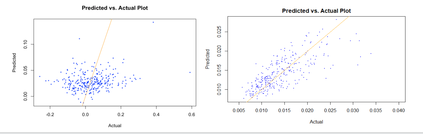
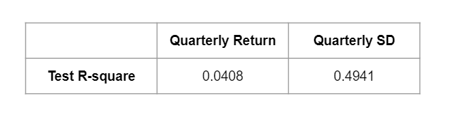
We visualize the predicted values and the actual values using a scatter plot to see the performance of our models. For predicting quarterly return, the dots are quite dispersed around the orange line. Negative returns were overestimated, positive returns were underestimated. And there are some outliers when return is too high, like above 0.4. As for predicting standard deviation, the dots are distributed a lot closer to the orange line, and our prediction was quite accurate, especially when the actual standard deviation is smaller than 0.022. But when the standard deviation is greater than 0.025, the model does not perform as well, and the residuals become larger. The visualization is consistent with the R-square for the two best models. While only four percent of the variance is explained by our model when predicting quarterly return, around 50% of the variance is explained when predicting quarterly standard deviation. Based on the performance results predicting the two target variables, it has been shown that predicting risk is much easier than predicting return.